Modeling System Leverages GIS to Assess Critical Assets

By Terry Martin

A “Sewer Pipe Risk Model” was developed by Seattle Public Utilities as a risk assessment tool to evaluate the city’s sewer and drainage assets using the existing GIS system. The model was created to provide a documented strategy for identification and management of high risk sewer and drainage pipes. The model interfaces directly with the city’s GIS system and extracts information pertaining to each pipe (i.e. elevation, installation date, material type, proximity to geologic features, etc.). It uses this information to calculate individual monetary consequences of failure and probabilities of failure based on these attributes. The model also predicts age-related probability of failure through the use of material and age-specific Weibull equations that are applied to each pipe in the City’s system.

Inspection of all sewer mains and storm drainage pipes is not a justifiable management strategy due to time and cost constraints. Prior to establishment of Seattle Public Utilities’ “Sewer Pipe Risk Model” the existing pipe inspection strategy used by the utility consisted of videotape inspection of each pipe in the system once every 30 years.

The network includes roughly 46,000 pipe runs, contains nearly 2,000 miles of pipe (with an average age of more than 70 years), and has an estimated worth of approximately $2.5 billion in 2004 dollars.

The 30-year return time for inspection was recently seen as inadequate for two primary reasons. Firstly, television inspections (via CCTV) performed infrequently seldom find failures before they occur. The return time was seen as too long to cost effectively anticipate and prevent failures on a consistent basis. Secondly, this CCTV practice focused too few resources on pipes which, when failure occurred, resulted in inordinately expensive or even catastrophic repair costs.

As an example, prior to implementation of the model a sewer pipe collapsed immediately downstream of a prominent local hospital in late 2002. This collapse resulted in an expensive repair as well as a substantial financial claim from the hospital. The broken pipe had not been video inspected since 1992 and was not scheduled to be assessed for another 20 years. This occurred despite the fact that the pipe was located amongst one of the oldest sections of infrastructure in the city and was subjected to historically high combined sewer/stormwater flows.

Seattle Public Utilities’ pipe inspection program now consists of an initial CCTV videotape inspection of all pipes found to be high risk by the model. After an initial inspection a high-risk pipe is placed on a CCTV review cycle of anywhere from two to 10 years based on the original condition assessment of the pipe. Variations in inspection frequency are employed in an effort to use limited CCTV resources in an efficient and cost-effective manner.

Determining the Annual Risk Cost of Failure

The decision to implement a condition-based maintenance program inherently depends on the relationship between the consequence of failure and the probability of failure. Formulas have been input into the model that calculate these factors, which comprise the basis of the “Sewer Pipe Risk Model.”

The risk cost of failure is represented by the following equation:
Risk Cost of Failure = Consequence of Failure x Probability of Failure

Consequence of Failure

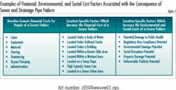
Table 1 shows some example multipliers used in the Risk Model to calculate the consequence of failure of a particular sewer pipe within Seattle’s system. The model interfaces directly with the city’s GIS system and extracts information pertaining to each pipe (i.e. elevation, installation date, material type, proximity to geologic features, etc.). It uses this information to calculate individual monetary consequences of failure based on these attributes. As an example, code was written into the model such that each pipe owned by Seattle Public Utilities which is located underneath a building is automatically affixed a multiplier of consequence based on the added cost of repairing a pipe located under a building.

The following is a short description of the cost factors shown in Table 1:

1) Baseline Generic Financial Costs for Repair of a Sewer Failure
The column on the left side of Table 1 shows the costs which consist of the estimated “hard” costs of repairing the pipe. Inputs for these variables have been estimated by comparing historical costs of similar repairs and applying these costs based on the depth, diameter, and material type of each pipe.

2) Location-Specific Factors Which Increase the Financial Cost of a Sewer Failure
The column in the center of Table 1 shows factors related to the consequences of failure which increase repair expenses based on the increase in complexity of performing repair work at a particular location. This added difficulty and expense of repair is taken into account using cost multipliers for repairs occurring in situations such as pipes located under bodies of water, under railroad tracks, under buildings, under freeways, within wetlands, on steep slopes, etc. The weighting of each factor has been determined using recent historical repair costs involving these characteristics. The current version of the model includes 18 separate multipliers of consequence including those that have been listed above.

3) Location-Specific Factors Which Increase the Environmental and Social Costs of a Sewer Failure
In addition to the aforementioned financial multipliers, the column on the right side of Table 1 shows other non-construction factors that may add to the cost of repairing a particular pipe. Monetary fines relating to regulatory non-compliance are one example of this classification of additive cost. Other examples of these costs include “intangible” (i.e. non-financial) costs such as potential damage to public health, environmental damage potential, unfavorable publicity potential, and property damage potential. The weighting of each of these factors has yet to be included in the model but will be included in subsequent versions.

Probability of Failure

The “Sewer Pipe Risk Model” accounts for the predictive probability of failure of a pipe in two ways. First, it uses location-specific cost multipliers similar to those discussed previously for the consequences of failure. As above, specific code was written to interface directly with the city’s GIS system and extract spatial and material information pertaining to each pipe. This information was used to calculate individual monetary effects of probability of failure. Examples include pipes exposed to adverse elements such as concrete pipes near force main outlets or at the bottom of steep slopes (damage from hydrogen sulfide gas), and proximity to liquefaction areas, steep slopes, hospitals, photographic processing facilities, or industrial locations which release pipe-damaging chemical constituents. The current version of the model includes eight such multipliers of probability. Future versions will also include location-specific water table and soil condition information affecting the probability of failure.

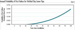
The second method by which probability of failure is determined is through the application of age-related failure prediction due to material degradation. The model applies a unique failure curve (based on normalized Weibull distribution) to each pipe in the system based on age and material type.

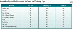
This method assumes that sewer pipes will display an approximately normal and exponential distribution of failure over time due to material breakdown. It assumes that no failures of this type occur earlier than 20 years after installation. As additional understanding is gained about life expectancy of the local piping network it is assumed that these curves will be modified to reproduce a more empirically based failure distribution curve for pipes unique to Seattle. Table 2 below summarizes model inputs for the various pipe materials in the City’s wastewater and drainage collection system.

Calculating Annual Risk Cost

Once the model has calculated a unique consequence of failure value for each pipe within the system this cost is multiplied by the unique probability of failure calculated for each pipe. The product is the total risk cost. The risk cost for each pipe is then annualized by incorporating the accumulated failure rate predicted by the Weibull curve for the current year plus five successive years. The time period of five years is used since this is the default CCTV return time for high-risk pipe condition assessment at Seattle Public Utilities. In this way the model evaluates the monetary risk borne by the utility for each pipe during the interim period between CCTV cycles.

Once the risk cost of failure is determined for an individual pipe this cost is compared to the net present value (NPV) of the lifecycle cost of video inspecting the particular pipe.

The net present value of the CCTV inspection lifecycle cost of a sewer pipe consists of initially determining the cost to videotape the pipe run a single time in current dollars. A discount rate is then applied to this cost as well as a frequency of video inspection of the pipe (i.e. once every five years) and a predetermined lifecycle length.

The following model inputs for net pressent value of the CCTV lifecycle costs were assumed:

1) A 5% discount rate was applied.
2) Each pipe run is video inspected once every five years.
3) The CCTV lifecycle length is 50 years.
4) Specific CCTV costs per lineal foot are based on historical values related to pipe diameter.

Cost multipliers for location within the city and depth of pipe were not applied.

Once the net present value of the CCTV inspection lifecycle cost is determined for each pipe it is compared to the risk cost of failure of the pipe run. Those pipes found to have a greater risk cost of failure than net present value of the CCTV inspection lifecycle cost (i.e. the benefit/cost ratio is greater than one) are considered to be high risk pipes.

Approximately 15% of the sewer pipes within the Seattle Public Utilities wastewater and drainage collection system were found to have a benefit/cost ratio exceeding one in the initial model run. Since the City currently CCTV videotapes approximately 3% of Seattle’s pipe inventory each year it was found that the amount of CCTV resources currently used was acceptable. However, as the model has shown, these resources were often misallocated in the past. A strategy shift has occurred whereby pipe assessment resources have now been changed from videotaping all of the pipes once every 30 years to videotaping only the high risk pipes an average of once every five years. It is expected that the 15% of pipes found to be high risk by the model will be assessed in the next five years without increasing CCTV resources. The remainder of pipes within the sewer and drainage collection system (approximately 85%) will be allowed to run to failure without condition assessment.

About the Author:
Terry Martin is the Wastewater and Drainage Lead for the Corporate Asset Management team at Seattle Public Utilities. SPU provides wastewater, drainage, and solid waste services to the citizens of Seattle as well as water service to the majority of the Greater Seattle Metropolitan Area. Martin is a registered Professional Civil Engineer, has worked for the Corporate Asset Management team at SPU for 2 ½ years, and has more than 13 years of public and private experience in the planning and design of municipal water, wastewater, and drainage infrastructure.